Objective

The main objective was to investigate the distribution and production of volatile halogenated organic compounds (halocarbons) in different habitats in the Arctic Ocean. Special emphasis was put on the contribution of halocarbons to the atmosphere produced by organisms in snow and ice compared with the contribution from pelagic organisms. Also, efforts were made to establish the importance of bacteria and cyanobacteria as producers of halocarbons.

Halocarbons are ubiquitous trace constituents of the oceans and the atmosphere. Their role in the global circulation of halogens and in atmospheric chemical reactions has been discussed extensively within the last few years in connection with their ability to affect the atmospheric ozone budget. Unlike the chlorofluorohydrocarbons (CFC’s), which are ozone depleting compounds of anthropogenic origin, other chlorinated, brominated and iodinated compounds are involved in a number of chemical and biological processes. It is known that a number of brominated and chlorinated compounds deliver chlorine and bromine to the stratosphere, and it has been shown that in the stratosphere, bromine is about 50 times more efficient in depleting ozone than is chlorine. It has also been shown that the synergistic effect of chlorine and bromine species accounts for approximately 20 % of the polar stratospheric ozone depletion. The iodinated substances have relatively short lifetimes in the atmosphere, and are therefore involved in reactions only in the lower troposphere.

The formation of halocarbons is presumed to be closely connected to the formation of hydrogen peroxide. We have suggested that during the reduction of hydrogen peroxide by haloperoxidases, halide ions are oxidised, thus forming hypochlorite and hypobromite, which will react with the dissolved organic matter, thus forming a number of halogen containing organic compounds.

In accordance with the objective the following studies have been performed:

• Studies of the production of halocarbons by pelagic, ice-living and snow microorganisms
• Studies of the surface water and air concentrations of halocarbons during transects
• Estimations of the flux of halocarbons from the sea surface to the atmosphere

Sampling strategy and analytical procedures

The project was part of leg 1 (Northwest Passage) and leg 3 (trans-Arctic). During leg 1, halocarbons were determined in surface sea water collected through the ship’s surface water inlet every hour from 59°30’N, 44°33’W (Cape Farewel) to 71°34’N, 156°17’W (Barrow). Air samples were collected continuously during this transect.

Sea water samples were collected from the rosette sampler along the transects during leg 3 (45 stations) for the determinations of halocarbons.

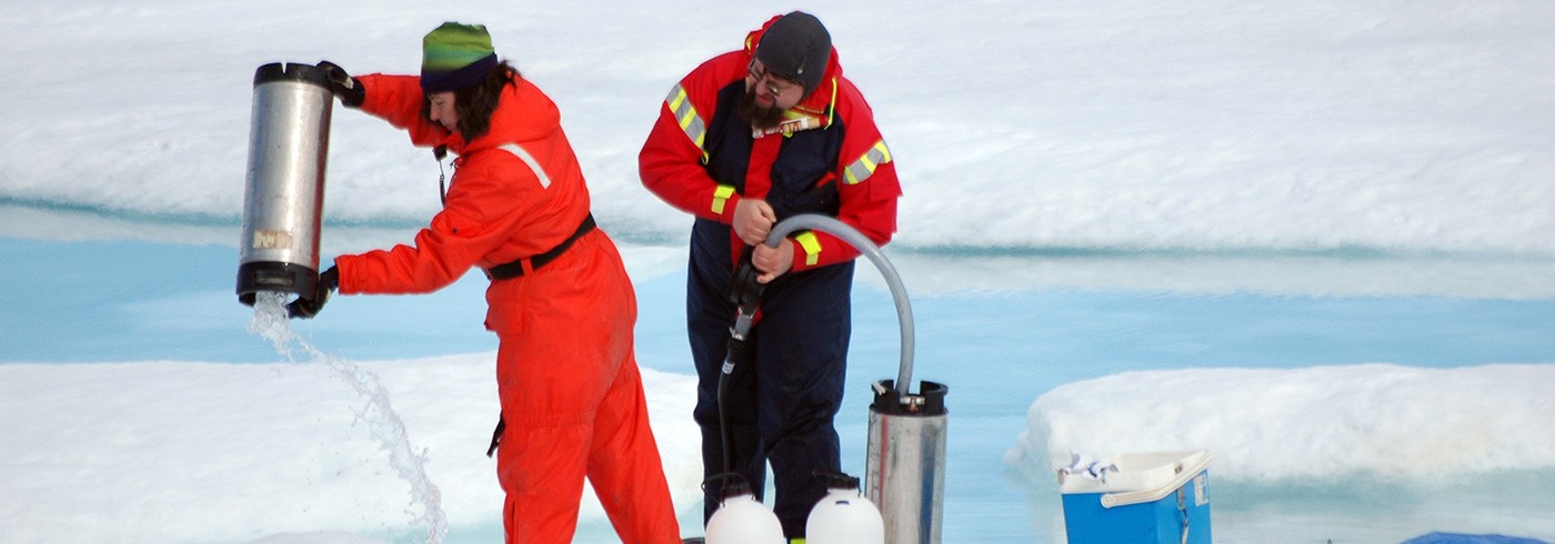
Fifteen ice stations were occupied during the cruise. During the stations brine was collected from several holes drilled in the ice, as well as water from underneath the ice, melt pond water and snow. The samples collected were used for incubation experiments onboard the ship. The experiments were performed in 60 ml glass bottles and incubated at +1°C and 150 µE. The production rates of halocarbons were determined and filters were stored in –80°C in order to determine pigment composition to relate the production rates of halocarbons to classes of organisms. The measurements of pigments will be performed in Uppsala with high performance liquid chromatography.

During the entire cruise air was sampled through a teflon tube. The air was drawn from the front of the ship at approximately a height of 12 m.

The halocarbons were pre-concentrated with a purge-and-trap technique, and then determined by capillary gas chromatography with either electron capture detection or mass spectrometric detection. The compounds measured were: iodomethane, iodoethane, 1-iodopropane, 2-iodopropane, 1-iodobuthane, 2-iodobuthane, diiodomethane, dibromomethane, tribromomethane, dibromochloromethane, bromodichloromethane, bromochloromethane, chloroiodomethane, dichloromethane, trichloromethane, trichloroethene and tetrachloroethene.

The photosynthetic rate and identification of classes of microorganisms were performed in all samples collected during ice stations with a Pulse Amplified Modulator (PAM).

Preliminary Results

Several factors are uncertain in the estimate of the emissions of halocarbons from the oceans to the atmosphere. It has been shown earlier that there are seasonal as well as geographical and diurnal differences in the production of halocarbons by marine algae. In addition, earlier studies have shown that there is a large release of halocarbons during spring in the Arctic, and it has been discussed if this “burst” is due to abiotic or biotic factors. During the Arctic Ocean 2002 expedition to the East Greenland Sea our investigations clearly demonstrated that the formation of halocarbons were predominantly taking place in sea ice and in snow, and that organisms occupying brine of high salinity were the most efficient producers.

Air–Sea flux measurements

Sea surface samples were collected every hour during the transit from Göteborg to Barrow, and air samples were measured continuously and these data are presently being evaluated. The observed increase of tribromomethane correlated well with the passages through heavy ice with the highest concentrations found in Peel Sound. Amazingly low concentrations of tribromomethane were found along the Canadian and Alaska coastline. The measured values corresponded to levels measured in waters of a depth larger than 2 000 m in the Canadian basin. The surface water concentrations of tetrachloromethane varied only slightly, which was expected.

Production of halocarbons in brine, snow and melt ponds

During leg 3 a number of experiments were performed in order to calculate the production rates of halocarbons formed in different environments. A production of halocarbons were measured in all experiments, and most surprisingly, halocarbons were formed in both melt ponds and snow (figure 1).

The preliminary results of measurements of photosynthesis with a Phyto/PAM in combination with light-microscopic observations showed that several species of green macroalgae, sometimes accompanied by cyanobacteria, dominated in the upper part of the sea ice layer (melt ponds, snow). When penetrating deeper into the ice the relative abundances of diatoms and dinoflagellates increased in the microalgal communities and these two groups fully dominated in the seawater just beneath the ice.

Another, more complicating, result was the observed spatial variability in the production rates. As can be seen in figure 2, the production rate of iodomethane varied significantly between two melt ponds situated not far from each other. To summarise, our results indicate that snow and melt ponds are active in the production of halocarbons. Since these habitats have a direct contact with the atmosphere, the amount of halocarbons produced will contribute to a large extent to the atmospheric content of halogenated compounds.