Accumulation of neurotoxic mercury (Hg) into the ice-covered Arctic
5 July 2005 - 10 October 2005
Left: Preliminary location of elevated DGM in surface water during leg 1.
Right: Preliminary distribution of volatile mercury along a vertical section of the Arctic Ocean.
Aim
It has been elucidated that high levels of neurotoxic mercury (Hg) in the Arctic are caused by a rapid, near-complete depletion of Hg in the atmospheric boundary-layer, occurring episodically during the polar spring (Schröder et al., 1998). Upon reaction with reactive bromine species (such as Br, BrO), hundreds of tons of Hg-II are perennially deposited on frozen surfaces. The relative magnitude of this sink is huge, resembling 30–40% of the current global deposition (Ariya et al., 2004). To some degree a back-reduction of Hg-II to Hg0 occurs, resulting in re-cycling of volatile mercury to the atmosphere (Sommar et al., 2004). However it can not compensate for the total deposition, and a net assimilation into the food chain occurs. The fate of Arctic mercury – after the enhanced deposition ending in May – is largely indefinite with reference to transport and transformation. The Beringia 2005 expedition, taking place a few months after the period of elevated deposition of mercury around the polar basin, offered an unique opportunity to sample vast until now unprobed exposed areas. The main objectives were to estimate the spread of mercury in the Arctic environment and to investigate the lability of the deposited Hg-II compounds with respect to reduction and methylation (to methyl-Hg).
Fieldwork
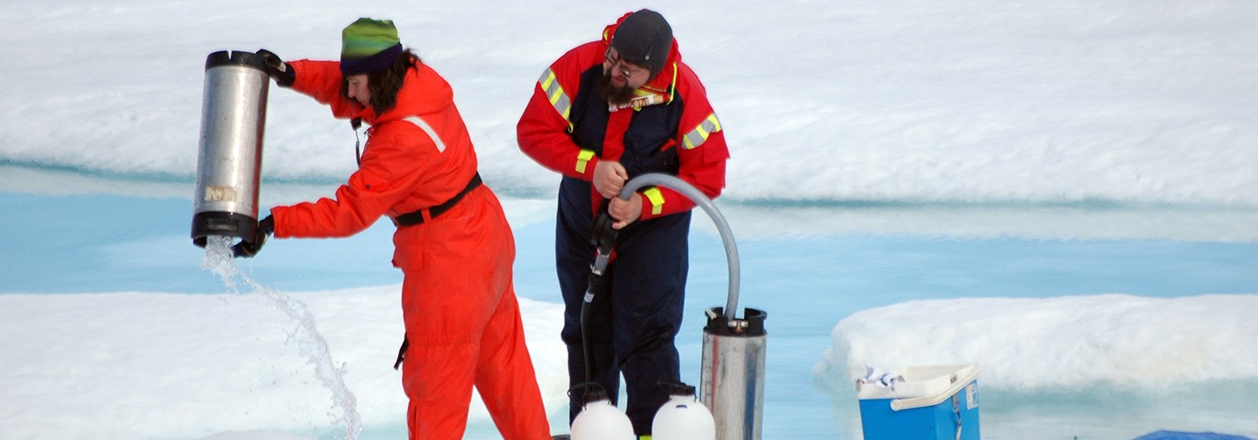
Using icebreaker Oden as a platform, continuous measurements of airborne mercury (mercury vapour and tiny fractions of Hg-II(g) and mercury species attached to particles (Hg-p)) and some related longlived gases (CO, O3) were performed during nearly three months en route. Automated instruments, with a time resolution of 10 minutes and less, sampled air taken well above the surrounding constructions. Surface water transferred to the main lab (on deck 1) was analysed continuously for dissolved mercury vapour (DGM) by using a method further developed from the equilibration device described in Gårdfeldt et al. (2002). By knowing the distribution of DGM in air and surface water, implicated one-sided outflow of mercury from the oceans can be quantified. The performance of the equilibration device was steadily positively verified on a single sample basis by stripping the mercury vapour from solution (manual method). DGM in other matrixes (vertical profiles of oceanic water, ice, snow and brine) was analysed by the manual method as well. Matching samples of mercury fractions (total-Hg and methyl-Hg) less sensitive for transformation were preserved by the addition of ultra-pure sulphuric acid and stored cold for future analysis. These three mercury fractions were sampled at about 55 stations generally comprising six depths vertically through the water column, most intense during the trans-polar section. With the help of expertise from the halocarbon group (Abrahamsson), vertically resolved brine samples within certain ice flows were obtained. In addition surface snow and melt pond water were probed. Our large set of samples is also made up of deep oceanic sediments obtained from the research group onboard USCGC Healy, intended for future analysis.
Preliminary results
The large number of samples collected have so far, for obvious reasons, only been analysed for their volatile mercury components (total-Hg and methyl-Hg remaining). However after extensive data processing and evaluation, we may on an incomplete basis report some interesting findings concerning volatile mercury.
Leg 1
Initially during the Atlantic transect we were able to establish the concentration levels of mercury vapour, carbon monoxide and ozone typical for the ambient midhemispheric background (figure 2). As can been seen in figure 2, several sharp features in CO and matching dips in the concentration of ozone are present in the running data. This is largely due to interception of emissions from the ship itself and is in general a marker for local combustion. From this perspective it is fortunate to observe that neither the concentrations of mercury in the gas-phase nor those attached to particles are notably influenced by the ship’s plume. On the contrary, strongly correlated elevated levels of mercury and carbon monoxide were observed in certain coastal industrialized destinations of the Beringia region (figure 2). The striking aspect of figure 2 is, however, the rapid increase of volatile mercury in surface water when entering ice-covered waters of the Canadian Arctic archipelago (e.g. Baffin Bay; see figure 1 to the left). The five to ten-fold increase in the surface-DGM causes strong supersaturation. When Oden breaks up the ice, as seen in figure 2, a fraction of the Hg0 pulse is spilled into the air samples. The Arctic Seas encountered with high DGM levels during Beringia 2005 essentially overlap with locations where observations of elevated BrO have been made from satellites (Richter et al., 2002). Interestingly, our novel data on DGM in the Arctic Seas will enable us to address and quantify the degree of recycling of mercury to the troposphere.

Temporal distribution of airborne Hg, O3 and CO as well as volatile mercury in surface water (not complete).
Leg 2–3
The data made available during the two more recent legs of the expedition comprise, in addition to air and surface water, ice and vertical ocean profiles. Analysis of DGM in ice samples (brine) frequently indicates levels that surpass those measured in the underlying surface sea water. In turn, along the trans-arctic oceanic section the highest levels of DGM were encountered in surface water, indicating the impact of the atmosphere and/or lightdriven chemistry (figure 1 to the right). From figure 1 an apparent inverse relation between DGM and the residence time of the water mass is implied. However, as we are lacking the distribution of total mercury at the time of writing, it appears presumptuous at this stage to say anything definite about this part of the arctic mercury cycle. Another issue worth looking into that turned up is the source distribution of arctic mercury. Moderate CO and Hg0 concentrations during the second part of August (sfigure 2) appear to coincide with prevailing atmospheric transport from Eurasia. By evaluating the Hg0/CO ratio we will hopefully be able to put constraints on the growing Asian emissions of mercury.